
QUANTIZATION OF THE HAMILTONIAN GOVERNING THE QUANTUM DYNAMICS OF ELECTRONS IN AN ELECTROMAGNETIC FIELD
Consider a non-relativistic charged particle in an electromagnetic field. As this post is to address the physics of electrons interacting with electromagnetic fields, the electric charge of the particle is taken to be \(-e\), where \(e = 1.602\times10^{-19}\,\mathrm{C}\) is the elementary charge. To describe particles with an arbitrary electric charge \(q\), simply perform the substitution \(e \rightarrow -q\) in the formulas you will subsequently encounter.
The task is to formulate the Hamiltonian governing the quantum dynamics of such a particle, subject to two simplifying assumptions: (i) the particle has charge and mass but is otherwise “featureless” (i.e., the spin angular momentum and magnetic dipole moment that real electrons possess are ignored), and (ii) the electromagnetic field is treated as a classical field, meaning that the electric and magnetic fields are definite quantities rather than operators.
Image source: Wikimedia Commons
License:Attribution-ShareAlike 4.0 International - CC BY-SA 4.0
Classically, the electromagnetic field acts on the particle via the Lorentz force law,
\[\mathbf{F}(\mathbf{r},t) = -e\Big(\mathbf{E}(\mathbf{r},t) + \dot{\mathbf{r}}\times \mathbf{B}(\mathbf{r},t)\Big),\]
where \(\mathbf{r}\) and \(\dot{\mathbf{r}}\) denote the position and velocity of the particle, \(t\) is the time, and \(\mathbf{E}\) and \(\mathbf{B}\) are the electric and magnetic fields. If no other forces are present, Newton’s second law yields the equation of motion
\[m\ddot{\mathbf{r}} = -e\Big(\mathbf{E}(\mathbf{r},t) + \dot{\mathbf{r}} \times \mathbf{B}(\mathbf{r},t)\Big), \label{eom}\]
where \(m\) is the particle’s mass. To quantize this, we must first convert the equation of motion into the form of Hamilton’s equations of motion.
Let us introduce the electromagnetic scalar and vector potentials \(\Phi(\mathbf{r},t)\) and \(\mathbf{A}(\mathbf{r},t)\):
\[\begin{align} \mathbf{E}(\mathbf{r},t) &= - \nabla \Phi(\mathbf{r},t) - \frac{\partial\mathbf{A}}{\partial t}, \\ \mathbf{B}(\mathbf{r},t) &= \nabla \times \mathbf{A}(\mathbf{r},t). \label{Bfield}\end{align}\]
We now postulate that the equation of motion \(\eqref{eom}\) can be described by the Lagrangian
Definition: Lagrangian
\[L(\mathbf{r},\dot{\mathbf{r}},t) = \frac{1}{2}m\dot{\mathbf{r}}^2 + e \Big[\Phi(\mathbf{r},t) - \dot{\mathbf{r}} \cdot \mathbf{A}(\mathbf{r},t) \Big]. \label{Lag}\]
This follows the usual prescription for the Lagrangian as kinetic energy minus potential energy, with \(-e\Phi\) serving as the potential energy function, except for the \(-e\dot{\mathbf{r}} \cdot \mathbf{A}\) term.
\[\frac{\partial L}{\partial r_i} = \frac{d}{dt} \frac{\partial L}{\partial \dot{r}_i}. \label{EulerLagrange}\]
The partial derivatives of the Lagrangian are:
\[\begin{align} \begin{aligned} \frac{\partial L}{\partial r_i} &= e\Big[\partial_i \Phi - \dot{r}_j \,\partial_i A_j \Big]\\ \frac{\partial L}{\partial \dot{r}_i} &= m\dot{r}_i - e A_i. \end{aligned}\end{align}\]
Now we want to take the total time derivative of \(\partial L /\partial \dot{r}_i\). In doing so, note that the \(\mathbf{A}\) field has its own \(t\)-dependence, as well as varying with the particle’s \(t\)-dependent position. Thus,
\[\begin{align} \begin{aligned} \frac{d}{dt} \frac{\partial L}{\partial \dot{r}_i} &= m\ddot{r}_i - e\, \frac{d}{dt} A_i(\mathbf{r}(t),t) \\ &= m\ddot{r}_i - e\, \partial_t A_i - e\, \dot{r}_j \partial_j A_i. \end{aligned}\end{align}\]
(In the above equations, \(\partial_i \equiv \partial/\partial r_i\), where \(r_i\) is the \(i\)-th component of the position vector, while \(\partial_t \equiv \partial/\partial t\).) Plugging these expressions into the Euler-Lagrange equations \(\eqref{EulerLagrange}\) gives
\[\begin{align} \begin{aligned} m\ddot{r}_i &= -e\Big[\Big(-\partial_i \Phi - \partial_t A_i\Big) + \dot{r}_j \Big( \partial_i A_j - \partial_j A_i\Big) \Big] \\ &= -e \Big[E_i(\mathbf{r},t) + \big(\dot{\mathbf{r}} \times \mathbf{B}(\mathbf{r},t) \big)_i\, \Big]. \end{aligned}\end{align}\]
(The last step can be derived by expressing the cross product using the Levi-Cevita symbol, and using the identity \(\varepsilon_{ijk} \varepsilon_{lmk} = \delta_{il} \delta_{jm} - \delta_{im} \delta_{jl}\).) This exactly matches Equation \(\eqref{eom}\), as desired.
We now use the Lagrangian to derive the Hamiltonian. The canonical momentum is
\[p_i = \frac{\partial L}{\partial \dot{r}_i} = m\dot{r}_i - e A_i. \label{canonp}\]
The Hamiltonian is defined as \(H(\mathbf{r},\mathbf{p}) = \mathbf{p} \cdot \dot{\mathbf{r}} - L\). Using Equation \(\eqref{canonp}\), we express it in terms of \(\mathbf{p}\) rather than \(\dot{\mathbf{r}}\):
\[\begin{align} \begin{aligned} H &= \mathbf{p}\cdot \left(\frac{\mathbf{p}+e\mathbf{A}}{m}\right) - \left(\frac{|\mathbf{p}+e\mathbf{A}|^2}{2m} + e\Phi - \frac{e}{m}(\mathbf{p}+e\mathbf{A})\cdot \mathbf{A}\right) \\ &= \frac{|\mathbf{p}+e\mathbf{A}|^2}{m} - \frac{e}{m}\mathbf{A}\cdot \left(\mathbf{p}+e\mathbf{A}\right) - \left(\frac{|\mathbf{p}+e\mathbf{A}|^2}{2m} + e\Phi - \frac{e}{m}(\mathbf{p}+e\mathbf{A})\cdot \mathbf{A}\right). \end{aligned}\end{align}\]
After cancelling various terms, we obtain
\[H = \frac{|\mathbf{p}+e\mathbf{A}(\mathbf{r},t)|^2}{2m} - e\Phi(\mathbf{r},t). \label{H0}\]
This looks a lot like the Hamiltonian for a non-relativistic particle in a scalar potential,
\[H = \frac{|\mathbf{p}|^2}{2m} + V(\mathbf{r},t).\]
In Equation \(\eqref{H0}\), the \(-e\Phi\) term acts like a potential energy, which is no surprise. More interestingly, the vector potential appears via the substitution
\[\mathbf{p} \rightarrow \mathbf{p} + e\mathbf{A}(\mathbf{r},t).\]
What does this mean? Think about what “momentum” means for a charged particle in an electromagnetic field. Noether’s theorem states that each symmetry of a system (whether classical or quantum) is associated with a conservation law. Momentum is the quantity conserved when the system is symmetric under spatial translations. One of Hamilton’s equations states that
\[\frac{dp_i}{dt} = \frac{\partial H}{\partial r_i},\]
which implies that if \(H\) is \(\mathbf{r}\)-independent, then \(d\mathbf{p}/dt = 0\). But when the electromagnetic potentials are \(\mathbf{r}\)-independent, the quantity \(m\dot{\mathbf{r}}\) (which we usually call momentum) is not necessarily conserved! Take the potentials
\[\Phi(\mathbf{r}, t) = 0, \;\;\; \mathbf{A}(\mathbf{r}, t) = Ct \hat{z},\]
where \(C\) is some constant. These potentials are \(\mathbf{r}\)-independent, but the vector potential is time-dependent, so the \(-\dot{\mathbf{A}}\) term in Equation \(\eqref{Bfield}\) gives a non-vanishing electric field:
\[\mathbf{E}(\mathbf{r},t) = - C\hat{z}, \;\;\;\mathbf{B}(\mathbf{r},t) = 0.\]
The Lorentz force law then says that
\[\frac{d}{dt}(m\dot{\mathbf{r}}) = eC\hat{z},\]
and thus \(m\dot{\mathbf{r}}\) is not conserved. On the other hand, the quantity \(\mathbf{p} = m\dot{\mathbf{r}} - e \mathbf{A}\) is conserved:
\[\frac{d}{dt}(m\dot{\mathbf{r}} - e\mathbf{A}) = eC\hat{z} - eC\hat{z} = 0.\]
Hence, this is the appropriate canonical momentum for a particle in an electromagnetic field.
We are now ready to go from classical to quantum mechanics. Replace \(\mathbf{r}\) with the position operator \(\hat{\mathbf{r}}\), and \(\mathbf{p}\) with the momentum operator \(\hat{\mathbf{p}}\). The resulting quantum Hamiltonian is
Definition: Quantum Hamiltonian
\[\hat{H}(t) = \frac{|\hat{\mathbf{p}}+e\mathbf{A}(\hat{\mathbf{r}},t)|^2}{2m} - e\Phi(\hat{\mathbf{r}},t). \label{quantumH}\]
Note
The momentum operator is \(\hat{\mathbf{p}} = -i\hbar\nabla\) in the wavefunction representation, as usual.
Gauge symmetry
The Hamiltonian \(\eqref{quantumH}\) possesses a subtle property known as gauge symmetry. Suppose we modify the scalar and vector potentials via the substitutions
\[\begin{align} \Phi(\mathbf{r},t) &\rightarrow \Phi(\mathbf{r},t) - \dot{\Lambda}(\mathbf{r},t) \label{gauge-subst-1} \\ \mathbf{A}(\mathbf{r},t) &\rightarrow \mathbf{A}(\mathbf{r},t) + \nabla{\Lambda}(\mathbf{r},t), \label{gauge-subst-2}\end{align}\]
where \(\Lambda(\mathbf{r},t)\) is an arbitrary scalar field called a gauge field. This is the gauge transformation of classical electromagnetism, which as we know leaves the electric and magnetic fields unchanged. When applied to the Hamiltonian \(\eqref{quantumH}\), it generates a new Hamiltonian
\[\hat{H}_\Lambda(t) = \frac{|\hat{\mathbf{p}}+e\mathbf{A}(\hat{\mathbf{r}},t) + e\nabla\Lambda(\hat{\mathbf{r}},t)|^2}{2m} - e\Phi(\hat{\mathbf{r}},t) + e\dot{\Lambda}(\hat{\mathbf{r}},t).\]
Now suppose \(\psi(\mathbf{r},t)\) is a wavefunction obeying the Schrödinger equation for the original Hamiltonian \(\hat{H}\):
\[i\hbar\frac{\partial\psi}{\partial t} = \hat{H}(t) \psi(\mathbf{r},t) = \left[\frac{|\hat{\mathbf{p}}+e\mathbf{A}(\hat{\mathbf{r}},t)|^2}{2m} - e\Phi(\hat{\mathbf{r}},t) \right]\psi(\mathbf{r},t).\]
Then it can be shown that the wavefunction \(\psi\, \exp(-ie\Lambda/\hbar)\) automatically satisfies the Schrödinger equation for the transformed Hamiltonian \(\hat{H}_\Lambda\):
\[i\hbar\frac{\partial}{\partial t} \left[\psi(\mathbf{r},t) \, \exp\left(-\frac{ie\Lambda(\mathbf{r},t)}{\hbar}\right)\right] = \hat{H}_\Lambda(t) \left[\psi(\mathbf{r},t) \, \exp\left(-\frac{ie\Lambda(\mathbf{r},t)}{\hbar}\right)\right]. \label{gaugeschrod}\]
To prove this, observe how time and space derivatives act on the new wavefunction:
\[\begin{align} \begin{aligned} \frac{\partial}{\partial t} \left[\psi \, \exp\left(-\frac{ie\Lambda}{\hbar}\right)\right] &= \left[\frac{\partial\psi}{\partial t} \;-\; \frac{ie}{\hbar} \dot{\Lambda}\, \psi \,\, \right] \exp\left(\frac{ie\Lambda}{\hbar}\right)\\ \nabla \left[\psi \, \exp\left(-\frac{ie\Lambda}{\hbar}\right)\right] &= \left[\nabla \psi - \frac{ie}{\hbar} \nabla \Lambda \,\psi \right] \exp\left(\frac{ie\Lambda}{\hbar}\right). \end{aligned}\end{align}\]
When the extra terms generated by the \(\exp(ie\Lambda/\hbar)\) factor are slotted into the Schrödinger equation, they cancel the gauge terms in the scalar and vector potentials. For example,
\[\begin{align} \Big(-i\hbar\nabla + e\mathbf{A} + e\nabla\Lambda\Big) \left[\psi \, \exp\left(-\frac{ie\Lambda}{\hbar}\right)\right] &= \Big[\left(-i\hbar\nabla + e\mathbf{A}\right)\psi\Big]\; \exp\left(-\frac{ie\Lambda}{\hbar}\right) \label{first_gauge_action}\end{align}\]
If we apply the \((-i\hbar\nabla + e\mathbf{A} + e\nabla\Lambda)\) operator a second time, it has a similar effect but with the quantity in square brackets on the right-hand side of \(\eqref{first_gauge_action}\) taking the place of \(\psi\):
\[\Big|-i\hbar\nabla + e\mathbf{A} + e\nabla\Lambda\;\Big|^2 \left[\psi \, \exp\left(-\frac{ie\Lambda}{\hbar}\right)\right] = \Big[\left|-i\hbar\nabla + e\mathbf{A}\right|^2\psi\Big]\; \exp\left(-\frac{ie\Lambda}{\hbar}\right).\]
The remainder of the proof for Equation \(\eqref{gaugeschrod}\) can be carried out straightforwardly.
The above result can be stated in a simpler form if the electromagnetic fields are static. In this case, the time-independent electromagnetic Hamiltonian is
\[\hat{H} = \frac{|\hat{\mathbf{p}}+e\mathbf{A}(\hat{\mathbf{r}})|^2}{2m} - e\Phi(\hat{\mathbf{r}}).\]
Suppose \(\hat{H}\) has eigenenergies \(\{E_m \}\) and energy eigenfunctions \(\{\psi_m(\mathbf{r})\}\). Then the gauge-transformed Hamiltonian
\[\hat{H}_\Lambda = \frac{|\hat{\mathbf{p}}+e\mathbf{A}(\hat{\mathbf{r}}) + e\nabla\Lambda(\mathbf{r})|^2}{2m} - e\Phi(\hat{\mathbf{r}})\]
has the same energy spectrum \(\{E_m\}\), with eigenfunctions \(\{\,\psi_m(\mathbf{r}) \exp[-ie\Lambda(\mathbf{r})/\hbar]\,\}\).
The Aharonov-Bohm effect
In quantum electrodynamics, it is the electromagnetic scalar and vector potentials that appear directly in the Hamiltonian, not the electric and magnetic fields. This has profound consequences. For example, even if a charged quantum particle resides in a region with zero magnetic field, it can feel the effect of nonzero vector potentials produced by magnetic fluxes elsewhere in space, a phenomenon called the Aharonov-Bohm effect.
A simple setting for observing the Aharonov-Bohm effect is shown in the figure below. A particle is trapped in a ring-shaped region (an “annulus”), of radius \(R\) and width \(d \ll R\). Outside the annulus, we set \(-e\Phi\rightarrow\infty\) so that the wavefunction vanishes; inside the annulus, we set \(\Phi = 0\). We ignore the \(z\)-dependence of all fields and wavefunctions, so that the problem is two-dimensional. We define polar coordinates \((r,\phi)\) with the origin at the ring’s center.
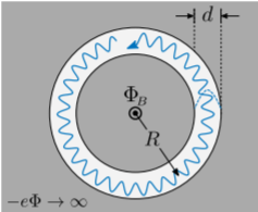
Now, suppose we thread magnetic flux (e.g., using a solenoid) through the origin, which lies in the region enclosed by the annulus. This flux can be described via the vector potential
\[\mathbf{A}(r,\phi) = \frac{\Phi_B}{2\pi r} \, \mathbf{e}_\phi, \label{Asolenoid}\]
where \(\mathbf{e}_\phi\) is the unit vector pointing in the azimuthal direction. We can verify from Equation \(\eqref{Asolenoid}\) that the total magnetic flux through any loop of radius \(r\) enclosing the origin is \((\Phi_B/2\pi r)(2\pi r) = \Phi_B\). The fact that this is independent of \(r\) implies that the magnetic flux density is concentrated in an infintesimal area surrounding the origin, and zero everywhere else. However, the vector potential \(\mathbf{A}\) is nonzero everywhere.
The time-independent Schrödinger equation is
\[\frac{1}{2m}\left|-i\hbar\nabla+ \frac{e\Phi_B}{2\pi r} \, \mathbf{e}_\phi\right|^2 \psi(r,\phi) = E\psi(r,\phi), \label{ABschrod}\]
with the boundary conditions \(\psi(R\pm d/2,0) = 0\). For sufficiently large \(R\), we can guess that the eigenfunctions have the form
\[\psi(r,\phi) \approx \begin{cases} \psi_0 \, \cos\left(\frac{\pi}{d}(r-R)\right)\, e^{i k R \phi}, & r \in [R-d/2, R + d/2] \\ 0 & \textrm{otherwise}. \end{cases}\]
This describes a “waveguide mode” with a half-wavelength wave profile in the \(r\) direction (so as to vanish at \(r = R \pm d/2\)), traveling in the azimuthal direction with wavenumber \(k\). The normalization constant \(\psi_0\) is unimportant. We need the wavefunction to be single-valued under a \(2\pi\) variation in the azimuthal coordinate, so
\[k \cdot 2\pi R = 2\pi n \;\;\;\Rightarrow \;\;\; k = \frac{n}{R}, \;\;\;\mathrm{where}\;\; n \in \mathbb{Z}.\]
Plugging this into Equation \(\eqref{ABschrod}\) yields the energy levels
\[\begin{align} E_n &= \frac{1}{2m} \left[ \left(\frac{n\hbar}{R} + \frac{e\Phi_B}{2\pi R}\right)^2 + \left(\frac{\pi\hbar}{d}\right)^2 \right] \\ &= \frac{e^2}{8\pi^2mR^2} \left(\Phi_B + \frac{nh}{e} \right)^2 + \frac{\pi^2\hbar^2}{2md^2}. \label{abcurves}\end{align}\]
These energy levels are sketched versus the magnetic flux \(\Phi_B\) in the figure below:

Each energy level has a quadratic dependence on \(\Phi_B\). Variations in \(\Phi_B\) affect the energy levels despite the fact that \(\mathbf{B} = 0\) in the annular region where the electron resides. This is a manifestation of the Aharonov-Bohm effect.
It is noteworthy that the curves of different \(n\) are centered at different values of \(\Phi_B\) corresponding to multiples of \(h/e = 4.13567\times10^{-5}\,\mathrm{T}\,\mathrm{m}^2\), a fundamental unit of magnetic flux called the magnetic flux quantum. In other words, changing \(\Phi_B\) by an exact multiple of \(h/e\) leaves the energy spectrum unchanged! This invariance property, which does not depend on the width of the annulus or any other geometrical parameters of the system, can be explained using gauge symmetry. When an extra flux of \(nh/e\) (where \(n\in\mathbb{Z}\)) is threaded through the annulus, Equation \(\eqref{Asolenoid}\) tells us that the change in vector potential is \(\Delta \mathbf{A} = (n\hbar/ e r) \mathbf{e}_\phi\). But we can undo the effects of this via the gauge field
\[\Lambda(r,\phi) = - \frac{n\hbar}{e} \, \phi \;\;\;\Rightarrow \begin{cases}\nabla \Lambda &= \displaystyle (n\hbar/er) \mathbf{e}_\phi \\ \displaystyle e^{-ie\Lambda/\hbar} &= \displaystyle e^{in\phi}. \end{cases}\]
Note that this \(\Lambda\) is not single-valued, but that’s not a problem! Both \(\nabla\Lambda\) and the phase factor \(\exp(-ie\Lambda/\hbar)\) are single-valued, and those are the quantities that enter into the gauge symmetry relations \(\eqref{gauge-subst-1}\)–\(\eqref{gauge-subst-2}\).